Web Performance Monitoring Metrics: Average, Percentiles, and SD

We are often asked what is the best metric to look at when monitoring web performance: average, percentiles, or standard deviation? It turns out that none of these are optimal, but that, depending on the type of measurement, either percentiles or standard deviations make good approximations.

Response, or the time it takes to load an HTTP request,  is never the same twice, of course: sometimes sites load fast, and sometime slow. It is the distribution of times which is of interest. The distribution tells us the probability of every possible response measurement: from 0s, to 1 ms, 2ms, and so on up to some cut off which we designate as “Too long.”

This distribution forms a picture (see below), from which we could calculate any probability we desired. Think of the bell-shaped curve of a normal distribution to get the idea.

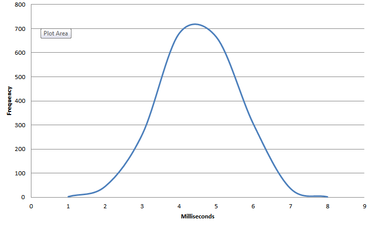
Storing and looking at complete distributions, especially for many different response measurements, can be very expensive and time consuming. Therefore, it would be nice if we had a way to quantify an approximation to a distribution.

Two methods exist, Percentiles and Standard Deviation.

Percentiles are, of course, just points along a distribution. The 50th percentile, or the Median, is that point which we expect 50% of the observations to be above, and 50% below. The 10th percentile is that point which we expect 10% of the points to be below, and the 90% percentile is that point which we expect 10% of the points to be above, 90% below.

If we laid out each (whole number) percentile—1 through 99—then we’d have a near perfect approximation of the entire distribution. But that is too many numbers to look at.   Typically, we’re only interested in the poor performers, so we pick a few top percentiles, like the 85th, 90th, 95th, and 99th.

Now suppose a particular response measurement is symmetric around its median.

A distribution is symmetric if each percentile less than the median, and 100 minus that percentile, are equidistant from the median.

For example, suppose the median was 2 seconds. Then, say, if the 10th percentile was 0.5 seconds, the 90th percentile should be 2.5 seconds.  We’d also have to have that if the 5th percentile was 0.1 seconds, the 95th percentile should be 3.9 seconds.  And so on for each other percentile.

In cases like these, or when symmetry is approximately true, the Average or Mean latency will equal the Median response. Then Standard Deviation can be used as a gauge of longer response times.   Standard deviation is just like it sounds: the routine deviation around the average.  For normal distributions, we know that roughly 70% of the responses will be within one standard deviation of the average; and that about 95% of the responses will be within two standard deviations.

For example, if we are comparing response measurements from the same URLs measured at different geographical locations, which we have determined are approximately symmetric with roughly equal averages, the one with the larger standard deviation will have longer response times.

But even if the two response measurements are symmetric, if they do not have roughly equal averages, then it is not clear which of the two will have longer response times, even if one has a higher standard deviations.

Here is an example from the same 5K image loaded from two separate locations, New York City and Miami utilizing Catchpoint’s web monitoring service. NYC is black, Miami orange. This is a picture of the full distribution of response times in milliseconds from over 4,000 measurements of each location: don’t miss the log axes. The medians have been indicated with dotted vertical lines: 3 ms for NYC, and 16 ms for Miami.

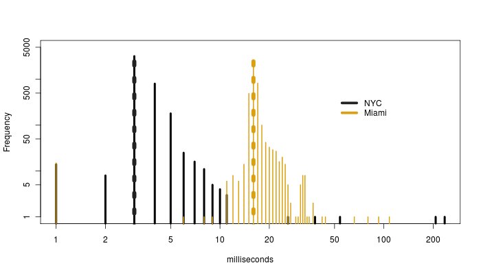
Neither of these distributions of response times are symmetric about their means, but the means are fairly close to the medians: 3.5 ms for NYC, 16.5 ms for Miami. The standard deviation is 4.9 ms for NYC, and 3.1 ms for Miami. If we didn’t have this picture, the reason for the differences in standard deviations would not be apparent unless we combined the means and standard deviations with the percentiles.

The danger of limited reports is apparent. The 95th and 99th percentiles are 5 ms and 7 ms for NYC and 19 ms and 25 ms for Miami. A first glance using the numbers thus far would indicate that Miami is slower. It isn’t until the 99.99th percentile that we see that NYC with 223 ms is much larger than Miami’s 101 ms. It is lose anomalous large values for NYC that drive up the standard deviation.

The answer to this article’s question is thus: no one metric is best. You are safer looking at a broad range of reports to come to a conclusion.

Special thanks to Matt Briggs for his contribution to this article. You can learn about Matt by visiting his site: http://wmbriggs.com/

Catchpoint Web Monitoring Solutions provide several metrics to build a full picture of you performance including: Average, Median, 85th Percentile, 95th Percentile, Standard Deviation, and Geometrical Mean. At Catchpoint Systems, we continuously listen to end users and talk to experts in the performance and monitoring fields, to better understand customer needs and figure out how to best solve them in our products.