Sampling Part 3: Subsampling & Non-uniform Sampling at Work

This is the last blog in the series on sampling. In the previous editions (Part I, Part IIa, and Part IIb), we had (a) provided an overview of the metrics arms race and had walked through the use of sampling in this regard, (b) overviewed margin of error associated with sampling and different types of sampling and (c) discussed the Simpson’s paradox. In this blog, we shall walk the audience through how subsampling [1] and non-uniform sampling [2] can be leveraged in the world of web operations.

Subsampling has a very rich research history. One of the early works can be traced to over five decades back, viz., Quenouille’s and Tukey’s jackknife. Mahalanobis suggested, albeit in a different context, the use of subsamples to estimate standard errors in studying crop yields, though he used the term interpenetrating samples. In [3, 4], Hartigan leveraged subsamples to construct confidence intervals and to approximate standard errors. Other use cases of subsampling include, but not limited to:

Variance estimation
Estimation of the underlying distribution

In the ops world, we mostly deal with time series data. This is exemplified by the plot below (the data was obtained using the Catchpoint portal).

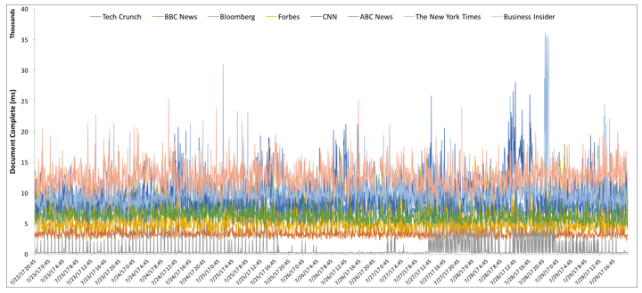
Given a time series, draw m observations without replacement. This constitutes one subsample. Repeat this N times. So, we have N subsamples, each of size m. Denote these subsamples by S1, S2, …, SN. Note that observations drawn for a subsample need not be contiguous. For instance, given a month long minutely time series, a subsample can potentially correspond to observations from the weekends. In a similar vein, one can create subsamples based on day of the week or hour-of-the-day and day-of-the-week (the latter would result in 168 non-overlapping subsamples).

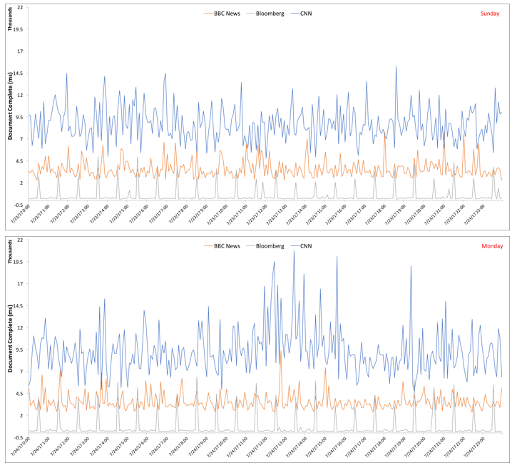
For instance, let’s consider two subsamples corresponding to a weekend day (Sunday) and a weekday (Monday) in the plot above. For ease of visualization, we limit the number of news outlets to three. The corresponding plots for the two days are shown below.

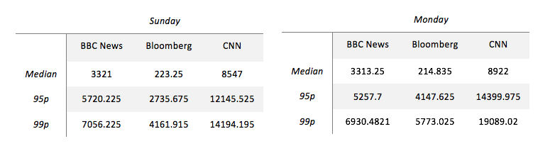
The tables below summarize the key stats for the plots above. From the tables, we note that, perhaps expectedly, 95p and 99p for Bloomberg and CNN is much higher on Monday than on Sunday. Surprisingly, for BBC News, all the three stats are in the same ballpark across Sunday and Monday. This may very well be an artifact of these two days and hence one should not generalize.

An analysis similar to the above can be done at the hour-of-the-day level. The insights learned can potentially serve as a valuable input to dynamic capacity planning.

Commonly used subsampling techniques cannot be used for time series data as they assume the observations to be i.i.d. (independent and identically distributed). This assumption clearly does not hold in the case of a time series data. Consequently, extensions to the traditional techniques for subsampling are needed.

A common approach to address the aforementioned limitation is to apply bootstrap to approximate i.i.d. setup by focusing on residuals of some general regression model. However, this approach is restricted to situations where a general regression model can be relied upon. In an ops context, it can be challenging to find a regression model to fit the data well – this stems from a wide variety of reasons such as, but not limited to, a non-normal distribution, heteroskedasticity. A more general approach is to resample the original data sequence by considering blocks of data rather than single data points as in the i.i.d. setup. The rationale behind the above is that within each block the dependence structure of the underlying model is preserved; further, if the block size is allowed to tend to infinity with the sample size, asymptotically correct inference can be made.

The blocking method mentioned above was employed by Carlstein for estimating variance of a general statistic. Specifically, he divided the original sequence in (non-overlapping) blocks of size b < n (where n is the total number of observations) and recomputed the statistic of interest on these blocks, and used the sample variance of the block statistics, after some suitable normalization. “Moving blocks” bootstrap [5, 6] can be used for, besides variance estimation, estimating the sampling distribution of a statistic so that confidence intervals or regions for unknown parameters can be constructed. Akin to Efron’s i.i.d. bootstrap, the method constructs pseudo-data sequences whose (known) data-generating mechanism follows the (unknown) data-generating mechanism that gave rise to the observed sequence. Having said that, the key difference lies in the fact that blocks of size b (< n), resampled with replacement from the data, are concatenated to form such a pseudo sequence rather than single data points. Note that in contrast to Carlstein’s approach, the moving blocks bootstrap uses overlapping blocks and is generally more efficient.

As discussed in earlier blog, it is common to measure multiple metrics to gauge performance and reliability. In a multivariate context such as this, a common problem is to draw simultaneous inference on the regression coefficients. Fortunately, subsampling can also be leveraged in higher dimensions. Last but not least, ops time series obtained from production are often non-stationary. Sources of non-stationarity are, for example, but not limited to, presence of seasonality, drift and an underlying trend. Several methods for subsampling from non-stationary time series have been proposed in the past. The reader is suggested to refer to Ch 4 of the book by Politis et al. [1].

It is not uncommon for metrics to be measured in production at different granularities, e.g., secondly, minutely et cetera. Further, there can be skew between time series (in other words, the multiple time series can be out of phase). Additionally, data may be missing in a time series – this may stem from a multitude of reasons such as, for instance, network error. The aforementioned inhibits carrying out of correlation analysis owing to different length of the time series. To this end, non-uniform sampling across metrics is often employed. Non-uniform sampling has been studied for over five decades in a wide variety of fields such as, but not limited to, signal processing, communication theory [7, 8], magnetic resonance imaging, astronomy, chemistry. In [12], Lüke remarked the following:

The numerous different names to which the sampling theorem is attributed in the literature – Shannon, Nyquist, Kotelnikov, Whittaker, to Someya – gave rise to the above discussion of its origins. However, this history also reveals a process which is often apparent in theoretical problems in technology or physics: first the practicians put forward a rule of thumb, then the theoreticians develop the general solution, and finally someone discovers that the mathematicians have long since solved the mathematical problem which it contains, but in “splendid isolation.

The roots of modern non-uniform sampling interpolation can be traced to the seminal work by Yen [9, 10]. In particular, he presented the interpolation formulas for special cases of irregular sampling such as migration of a finite number of uniform samples, a single gap in otherwise uniform samples and periodic non-uniform sampling. The reader is suggested to refer to the surveys by Jerri [11], Butzer et al. [12] or the book by Marvasti [1] for a deep dive into the subject of non-uniform sampling.

To summarize, subsampling and non-uniform sampling can come in handy (and in some case, are required) to extract actionable insights from ops time series data.

Readings

[1] “Subsampling“, by D. N. Politis et al.

[2] “Nonuniform Sampling: Theory and Practice“, by F. Marvasti (Ed.).

[3] “Using subsample values as typical values”, by J. Hartigan, 1969.

[4] “Necessary and Sufficient Conditions for Asymptotic Joint Normality of a Statistic and Its Subsample Values”, by J. Hartigan, 1975.

[5] “The jackknife and the bootstrap for general stationary observations”, by H. R. Kiinsch, 1989.

[6] “Moving blocks jackknife and bootstrap capture weak dependence”, by R. Y. Liu and K. Singh, 1992.

[7] “A Mathematical Theory of Communication”, by C. E. Shannon, 1948.

[8] “Communication in the Presence of Noise” by C. E. Shannon, 1949.

[9] “On Nonunifonn Sampling of Bandwidth-limited Signals”, by J. L. Yen, 1956.

[10] “On the synthesis of line-sources and infinite strip-sources”, by J. L. Yen, 1957.

[11] “The Shannon Sampling Theorem – its Various Extension and Applications: A Tutorial”, by A. J. Jerri, 1977.