Blog post
Blog Post
Sampling Part IIa: Types and Example Use Cases
Part 2a of our sampling series will explore various types and examples use cases. Read this blog for more sampling tips.
In Part I, we provided an overview of the metrics arms race and had walked through the use of sampling in this regard. We had also discussed the importance of baking in recency of data during sampling and some of the pitfalls of sampling such as the sampling error. Recall that exact measurement of sampling error is not feasible as the true population values are generally unknown; hence, sampling error is often estimated by probabilistic modeling of the sample.
Random sampling error is often measured using the margin of error statistic. The statistic denotes a likelihood that the result from a sample is close to the number one would get if the whole population had been used. When a single, global margin of error is reported, it refers to the maximum margin of error using the full sample. Margin of error is defined for any desired confidence level; typically, a confidence of 95% is chosen. For a simple random sample from a large population, the maximum margin of error, Em, is computed as follows:
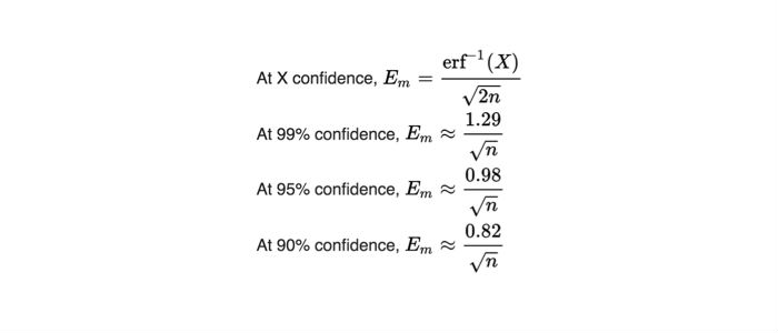
where, erf is the inverse error function and n is the sample size. In accord to intuition, maximum margin of error decreases with a larger sample size. It should be noted that margin of error only accounts for random sampling error and is blind to systematic errors.
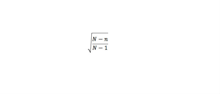
An underlying assumption of the formula above for the margin of error is that there is an infinitely large population and hence, margin of error does not depend on the size of the population (N) of interest. Given the real-time large volume of operational data, the assumption can be assumed to hold for practical purposes. Having said that, the aforementioned assumption is valid when the sampling fraction is small (typically less than 5%). On the other hand, if no restrictions – such as that n/N should be small, or N large, nor that the latter population is normal – are made, then, as per Isserlis, the margin or error should be corrected using the following:
It is important to validate the underlying assumptions as sampling error has direct implications on analysis such as anomaly detection (refer to Part I).
The following sampling methodologies have been extensively studied and used in a variety of contexts:
- Simple Random Sampling: It is a method of selecting n units out of N such that every one of the NCn samples has an equal chance of being drawn. Random sampling can be done without or with replacement.
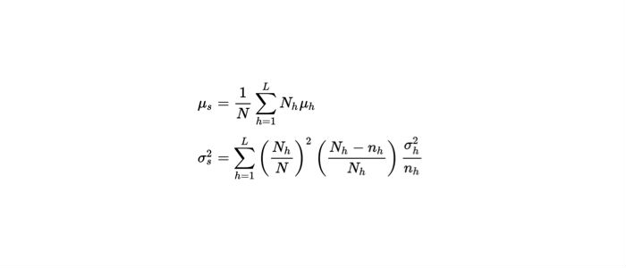
- Stratified Random Sampling: Under this method, the overall population is divided into sub-populations (or strata) such that they are non-overlapping and collectively exhaustive. Then, a random sample is drawn from each strata. The mean and variance of stratified sampling are given as follows:
where,
N= Population size
L = # strata
Nh = Size of each stratum
nh = Size of random sample drawn from statum h
sh = sample standard deviation of stratum h
mh = sample mean of stratum h
This often improves the representativeness of the sample by reducing sampling error. On comparing the relative precision of Simple Random and Stratified Random Sampling, Cochran remarked the following:
… stratification nearly always results in smaller variance for the estimated mean or total than is given by a comparable simple random sample. … If the values of nh are far from optimum, stratified sampling may have a higher variance.
where, nh is the size of a random sample from a stratum.
In the context of operations, let’s say that if one were to evaluate the Response Time of a website, the response time data should be divided into multiple strata based on geolocation and then analyzed.
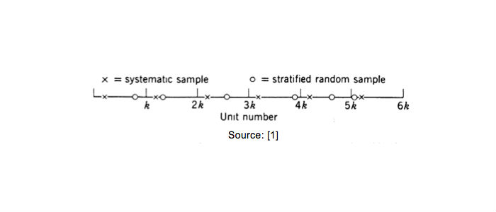
- Systematic Sampling: In this method, a unit is sampled from the first k units and then every k-th unit is sampled thereafter. For example, if k=10 and the first unit sample if 7, then units numbered 17, 27, … are sample subsequently. This method is also referred to as every k-th systematic sample. A visual comparison between systematic sampling and stratified random sampling is shown below:
A variant of the above sets the start of the sampling sequence to (k+1)/2 if k is odd or to k/2 is k is even. In another variation, the N units are assumed to be arranged around a circle, a number between 1 and N is selected at random and then every k-th (where k = integer nearest to N/n) unit is sampled. The reader is referred for further reading on systematic sampling.
- Adaptive Sampling: Under this method, the sampling strategy is modified in real time as data collection occurs – based on the information gathered from previous sampling that has been completed. Adaptive sampling is frequently used in the context of databases, e.g., estimating the size of a query. It also finds applications in the world of web operations. For instance, if one were to monitor the performance of a website, uniform sampling of response time would not shed light on potential issue during periods of high traffic. To alleviate this, the sampling rate should be adapted to the incoming traffic. Specifically, during periods of high traffic, the sampling rate should be increased; likewise, during periods of low traffic, the sampling rate should be decreased.
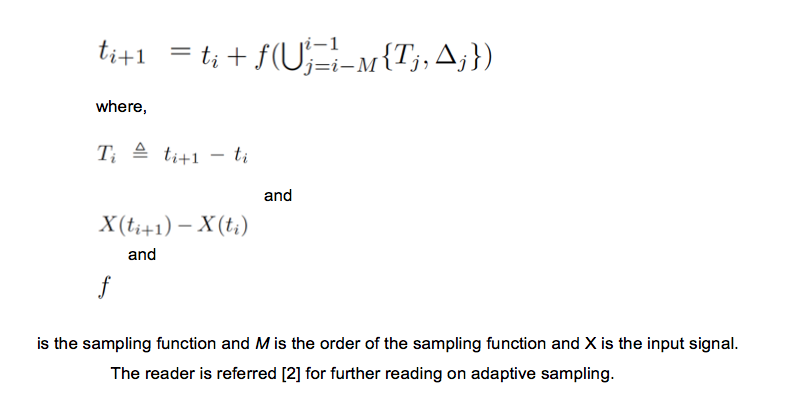
Several variants of adaptive sampling have been proposed in the literature. For instance, in Locally Adaptive Sampling, intervals between samples is computed using a function of previously taken samples, called a sampling function. Hence, though it is a non-uniform sampling scheme, one need not keep sampling times. In particular, sampling time ti+1 is determined in the following fashion:
We now walk through a couple of examples to illustrate the applicability of the sampling techniques discussed above. The plot below compares # Page Views across the different continents over a three-day period. The data was collected every hour. Note that the scale of the y-axis is logarithmic.
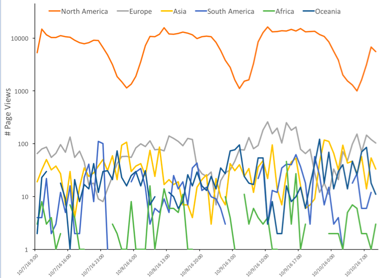
Simple random or stratified random sampling of the time series in the plot above would render the subsequent comparison inaccurate owing to the underlying seasonality. This can be addressed by employing systematic sampling whereby #page views of the same hour for each day would be sampled. Subsequent comparison of the sampled data across different continents would be valid.
The plot below compares Document Completion time across the different continents over a three-day period. The data was collected every hour. Note that the scale of the y-axis is in thousands of milliseconds. From the plot we note that, unlike # Page Views, Document Completion time does not exhibit a seasonal nature.
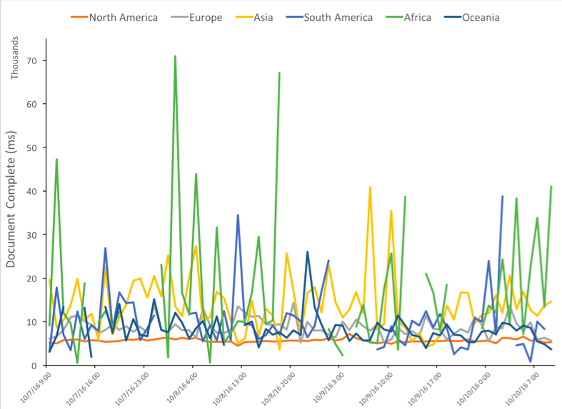
Given the high variance of the Document Completion time, employing simple random sampling would incur a large sampling error. Consequently, in this case stratified random sampling – where a stratum would correspond to a day – can be employed and then the sampled data can be used for comparative analysis across the different continents.
Readings
[1] “Sampling techniques”, W. G. Cochran.
[2] “Adaptive Sampling”, Steven K. Thompson, George A. F. Seber
By: Arun Kejariwal, Ryan Pellette, and Mehdi Daoudi
November 4, 2016


Catchpoint Team
This is some text inside of a div block.